Intro
Probabilistic models are ubiquitous in statistics and machine learning. The computational challenges surrounding statistical inference often force these models to be exceedingly simple. Consequently, a central goal is to improve model specification by making it feasible to use more realistic descriptions of data generating processes.
Normalizing flows provide a mechanism to transform simple distributions into more complex ones without sacrificing the computational conveniences that make the former appealing and practical.
The idea was introduced in its popular form to the machine learning community in Rezende et al.
In that paper, the authors begin their demonstration of the expressivity of normalizing flows by approximating several non-Gaussian toy densities.
In this post I’ll go over a minimal implementation of normalizing flows using PyTorch to try and replicate this result. The goal is to gain a better understanding of how normalizing flows work and are used. All the code can be found on Github.
Context
Normalizing flows are a general tool to express probability distributions, but their utility is exemplified in the context of variational inference (VI). For an in depth review of this subject some great references are: Variational Inference: A Review for Statisticians, or Graphical Models, Exponential Families, and Variational Inference.
Variational Inference
A brief refresher of VI, following Blei et al:
Consider a joint distribution $p(z, x) = p(z) p(x|z)$ with latent variables $\mathbb{z}=z_{1:m}$ and observations $\mathbb{x}=x_{1:n}$ With $z \sim p(\mathbb{z})$. Bayes’ rule then relates the data and the posterior $p(z|x)$ as follows:
$p(z|x)\propto p(z)p(x|z)$
Normalizing the R.H.S is often intractable (unfeasible) and so approximate inference is needed.
Variational inference achieves this by using a simpler family of distributions $\mathcal{D}$ over the latent variables as an approximation. The parameters of the simpler distributions (the variational parameters) are then optimized to be as “good” as possible. The quality of the approximation is usually measured using the Kullback–Leibler (KL) divergence from the true posterior:
$q^{*}(z)= argmin_{q(x)\in \mathcal{D}} KL(q(z) || p(z|x))$
There’s a lot more to be said here, but the role of normalizing flows in this context is already clear. If our variational family is too simple, even the optimal setting of the variational parameters could result in a unusable approximation that is “far” from the true posterior.
Normalizing flows
The basic idea is to pass a sample from a simple base distribution through a series of transformations or flows. The transformations $f$ must be smooth, differentiable ($f$ and $f^-1$) and invertible. Functions of this type are known as diffeomorphisms. The transformed sample can now be thought of as a sample from a more complex distribution. The invertibility condition gives a closed form description of the relationship between the density of the initial distribution and the final.
Consider an invertible smooth mapping $$f: \mathcal{R}^{d} \to \mathcal{R}^d$$ with an inverse $f^{-1} = g$.
Given a random variable $\mathbb{z}$ with distribution $q(\mathbb{z})$, $\mathbb{z}^{'} = f(\mathbb{z})$ has the distribution:
$$q(\mathbb{z}') = q(\mathbb{z}) |det \frac{\partial f^{-1}}{\partial \mathbb{z}^{'}} | = q(\mathbb{z})| det \frac{\partial f}{\partial \mathbb{z}} |^{-1}$$
Additionally if we use $k$ flows and transform our initial sample $\mathbb{z}_0$: $\mathbb{z}_k= f_K \circ … \circ f_2 \circ f_1(\mathbb{z}_0)$
We can get the final log-density $\ln(q_k(\mathbb{z}))$ as follows:
$\ln q_K(\mathbb{z}_K)= \ln_{q_0}(\mathbb{z}_0)-\sum_{k=1}^K \ln \lvert det \frac{\partial f_k}{\partial \mathbb{z}_{{k-1}}}\rvert$
Nice!
Now all we need is an invertible transformation to use. The authors propose a family of transformations called planar flows which take the form: $$f(z)=z+uh(w^T z + b)$$ Where:
- $\mathbb{w} \in \mathcal{R}^D$
- $\mathbb{u} \in \mathcal{R}^D$
- $b \in \mathcal{R}$
- $h$ is an elementwise nonlinearity (like tanh).
The Determinant-Jacobian can be computed efficiently:
$$\psi(\mathbb{z}) = h’(\mathbb{w}^Tz + b)\mathbb{w}$$ $$| det \frac{\partial f}{\partial \mathbb{z}}| = \lvert 1+ \mathbb{u}^T \psi(\mathbb{z}) \rvert $$
Our formula for the final log density is:
$$\ln q_K(\mathbb{z}_K) = \ln_{q_0}(\mathbb{z}) - \sum_{k=1}^K \ln \lvert 1 + \mathbb{u}_k^T \psi_k(\mathbb{z}_{k-1})\rvert$$
Potential functions
The paper proposes four potential functions $U(z)$ with unnormalized densities $p(\mathbb{z}) \propto exp[-U(\mathbb{z})]$
This is what they look like evaluated in the range $(-4, 4)^2$: 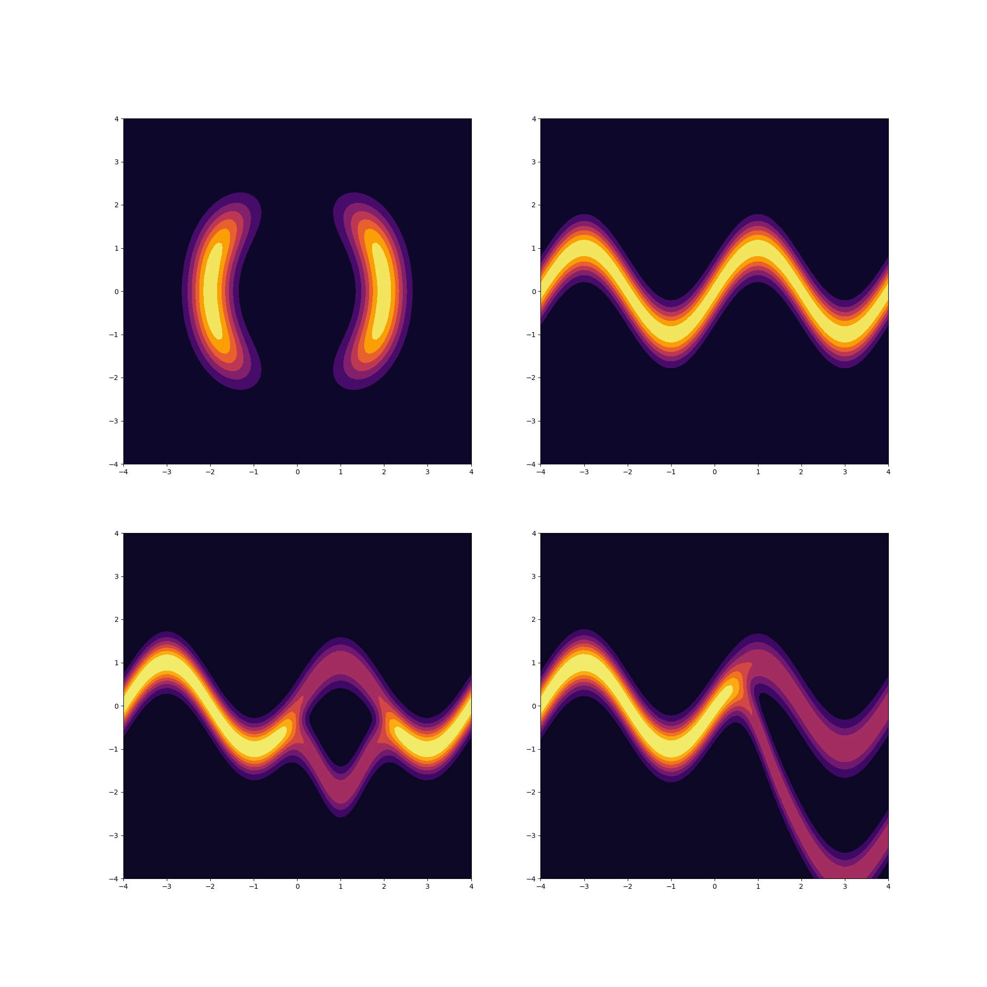
What we’re optimizing
Since we can evaluate the target density but can’t sample from it we minimize the reverse KL divergence as described in Papamakarios et al.
For clarity consider the following formulation:
- Our transformation $T$ with params $\phi$
- Our base distribution $p(\mathbb{u})$ with params $\psi$,
- The target distribution $p^*(\mathbb{x})$
the reverse KL is:
$$E_{p_{u}(\mathbb{u}; \psi)} [- \log p^*(\mathbb{x})(T(\mathbb{u};\phi)) - \log |det J_T(\mathbb{u}; \phi)| + \log p_u(\mathbb{u}; \psi)] $$
$\log p_u(u; \psi)$ doesn’t change so we can ignore it.
Implementation
We can implement our target densities as simple functions that take a 2-D point and return a scalar value. For example, take the code for the first example in the figure above:
def w_1(z):
    return torch.sin((2 * math.pi * z[:, 0]) / 4)


def w_2(z):
    return 3 * torch.exp(-.5 * ((z[:, 0] - 1) / .6) ** 2)


def sigma(x):
    return 1 / (1 + torch.exp(- x))


def w_3(z):
    return 3 * sigma((z[:, 0] - 1) / .3)


def pot_1(z):
    z_1, z_2 = z[:, 0], z[:, 1]
    norm = torch.sqrt(z_1 ** 2 + z_2 ** 2)
    outer_term_1 = .5 * ((norm - 2) / .4) ** 2
    inner_term_1 = torch.exp((-.5 * ((z_1 - 2) / .6) ** 2))
    inner_term_2 = torch.exp((-.5 * ((z_1 + 2) / .6) ** 2))
    outer_term_2 = torch.log(inner_term_1 + inner_term_2 + 1e-7)
    u = outer_term_1 - outer_term_2
    return - u
Next we need to implement a planar flow. A planar flow needs to be able to transform a given sample $T(x)$ and return the computed log determinant of the Jacobian.
class PlanarFlow(nn.Module):
    """
    A single planar flow, computes T(x) and log(det(jac_T)))
    """
    def __init__(self, D):
        super(PlanarFlow, self).__init__()
        self.u = nn.Parameter(torch.Tensor(1, D), requires_grad=True)
        self.w = nn.Parameter(torch.Tensor(1, D), requires_grad=True)
        self.b = nn.Parameter(torch.Tensor(1), requires_grad=True)
        self.h = torch.tanh
        self.init_params()

    def init_params(self):
        self.w.data.uniform_(-0.01, 0.01)
        self.b.data.uniform_(-0.01, 0.01)
        self.u.data.uniform_(-0.01, 0.01)

    def forward(self, z):
        linear_term = torch.mm(z, self.w.T) + self.b
        return z + self.u * self.h(linear_term)

    def h_prime(self, x):
        """
        Derivative of tanh
        """
        return (1 - self.h(x) ** 2)

    def psi(self, z):
        inner = torch.mm(z, self.w.T) + self.b
        return self.h_prime(inner) * self.w

    def log_det(self, z):
        inner = 1 + torch.mm(self.psi(z), self.u.T)
        return torch.log(torch.abs(inner))
Finally we want a class to compose multiple planar flows. Given a sample it ought to sequentially apply the flows and return the summed log determinant-Jacobians.
class NormalizingFlow(nn.Module):
    """
    A normalizing flow composed of a sequence of planar flows.
    """
    def __init__(self, D, n_flows=2):
        super(NormalizingFlow, self).__init__()
        self.flows = nn.ModuleList(
            [PlanarFlow(D) for _ in range(n_flows)])

    def sample(self, base_samples):
        """
        Transform samples from a simple base distribution
        by passing them through a sequence of Planar flows.
        """
        samples = base_samples
        for flow in self.flows:
            samples = flow(samples)
        return samples

    def forward(self, x):
        """
        Computes and returns the sum of log_det_jacobians
        and the transformed samples T(x).
        """
        sum_log_det = 0
        transformed_sample = x

        for i in range(len(self.flows)):
            log_det_i = (self.flows[i].log_det(transformed_sample))
            sum_log_det += log_det_i
            transformed_sample = self.flows[i](transformed_sample)

        return transformed_sample, sum_log_det
Optimization
Taking this all together we can iteratively update the parameters using stochastic gradient descent.
- Sample from the base distribution (Gaussian)
- Apply the sequence of flows to the sample and get the sum of log determinant Jacobians
- Evaluate the loss (reverse KL)
- Compute the gradient and update the parameters
model = NormalizingFlow(2, args.N_FLOWS)

# RMSprop is what they used in renzende et al
opt = torch.optim.RMSprop(
    params=model.parameters(),
    lr=args.LR,
    momentum=args.MOMENTUM
)

scheduler = ReduceLROnPlateau(opt, 'min', patience=1000)
losses = []

for iter_ in range(args.N_ITERS):
    if iter_ % 100 == 0:
        print("Iteration {}".format(iter_))

    samples = Variable(random_normal_samples(args.BATCH_SIZE))

    z_k, sum_log_det = model(samples)
    log_p_x = target_density(z_k)

    # Reverse KL since we can evaluate target density but can't sample
    loss = (- sum_log_det - (log_p_x)).mean()

    opt.zero_grad()
    loss.backward()
    opt.step()
    scheduler.step(loss)

    losses.append(loss.item())

    if iter_ % 100 == 0:
        print("Loss {}".format(loss.item()))
Results
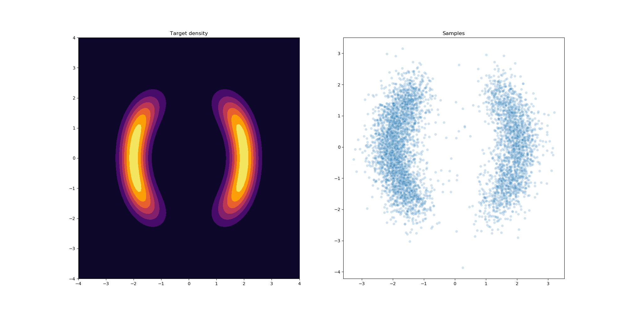
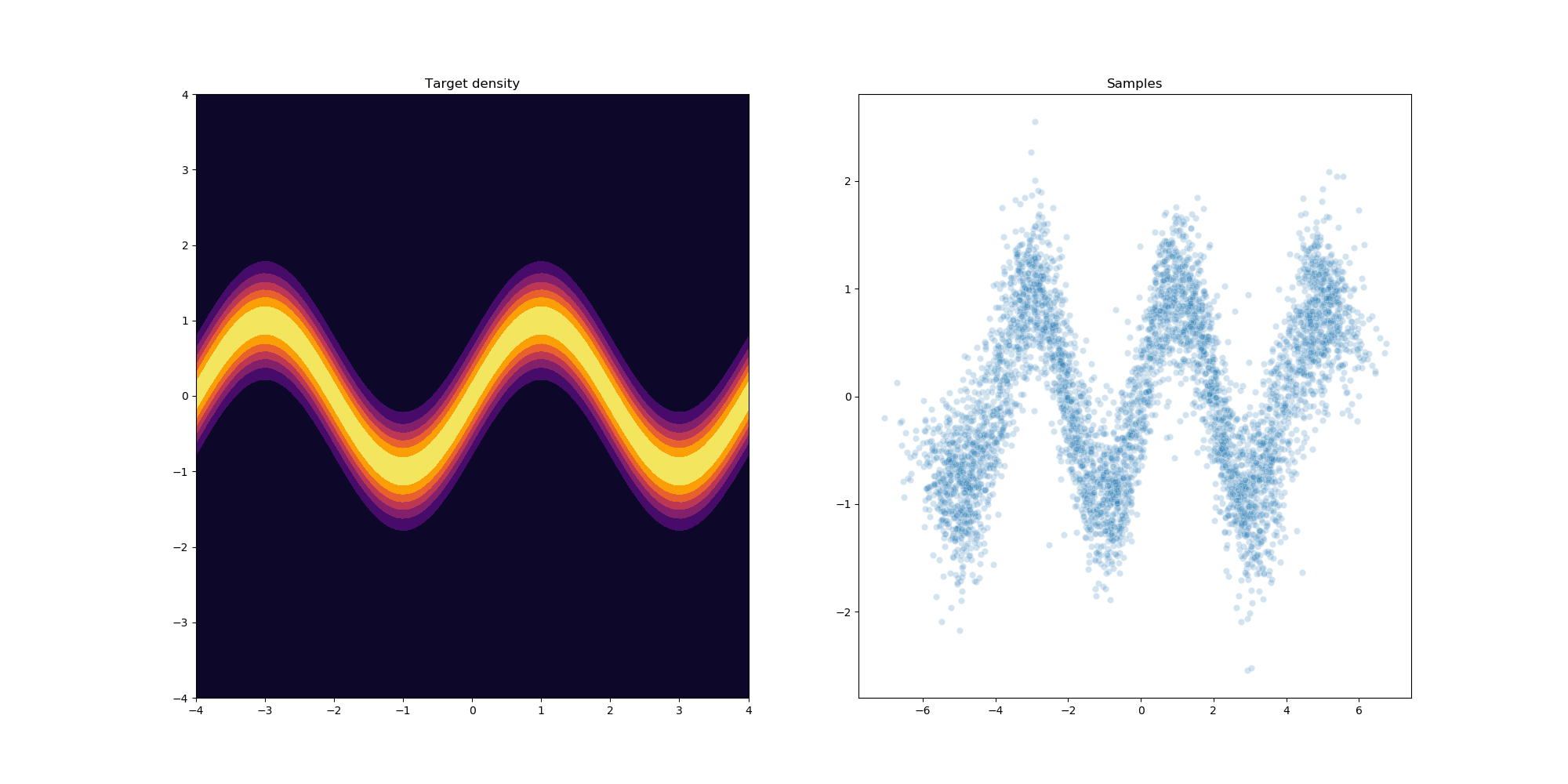
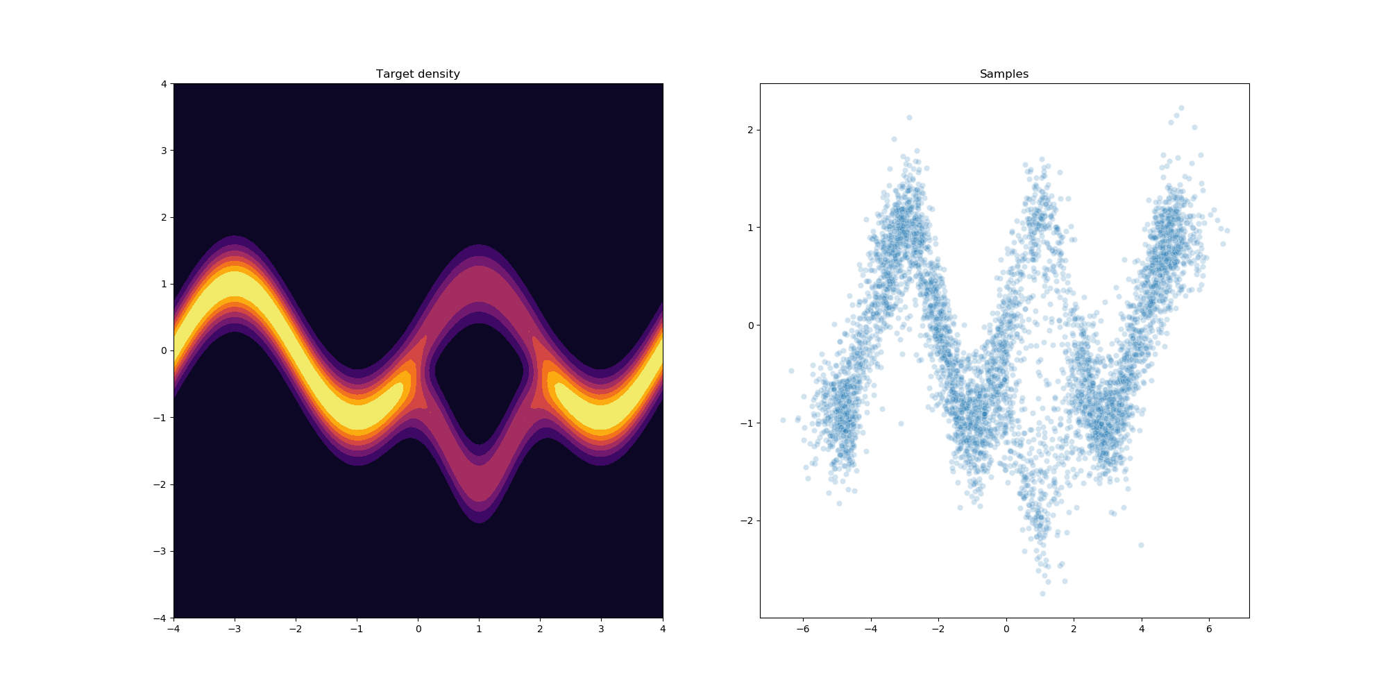
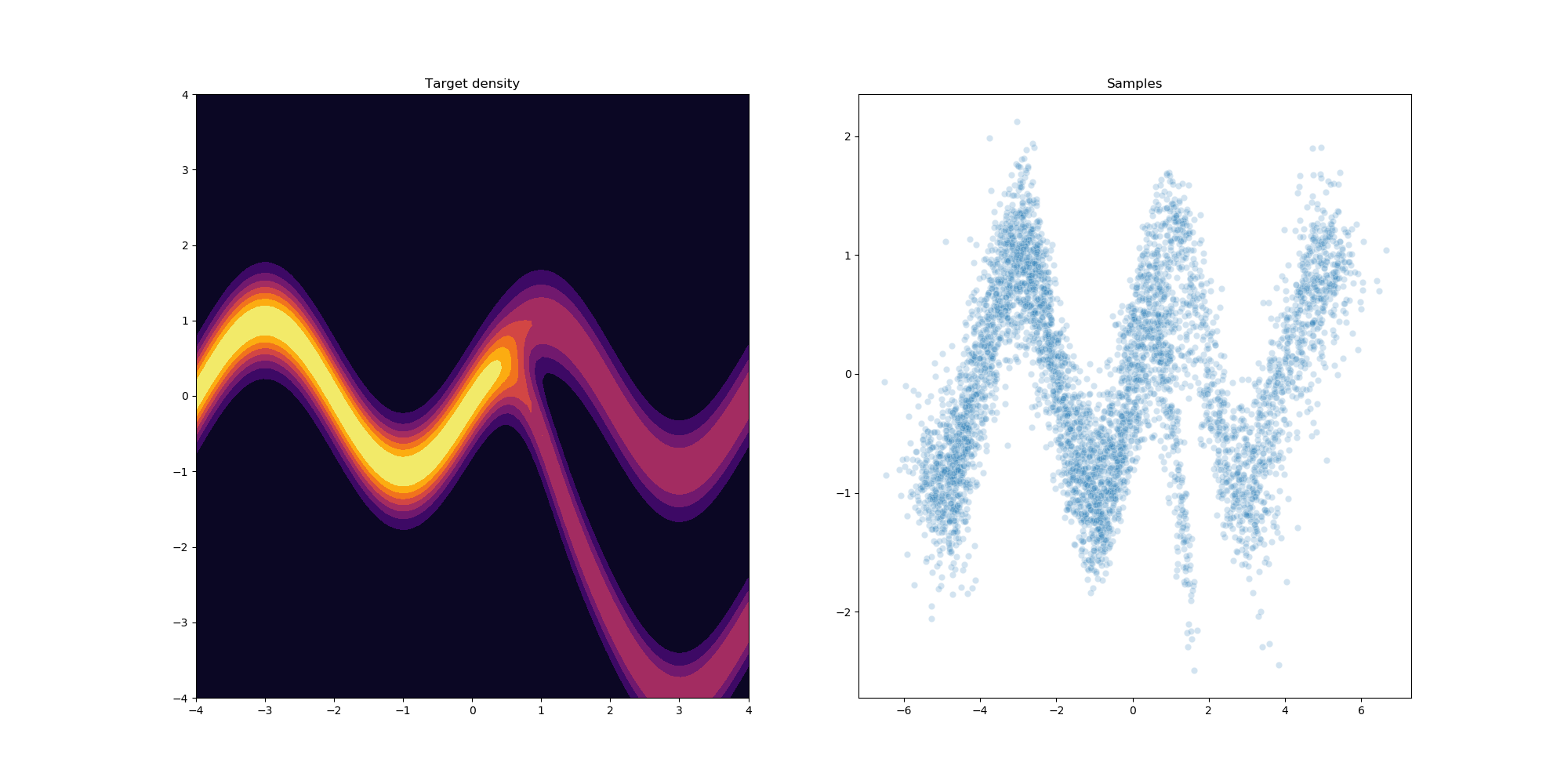
After a little bit of hyperparameter optimization of the number of flows and learning rate we can get the following results using 32 planar flows.
References
Blei, David M., Alp Kucukelbir, and Jon D. McAuliffe. “Variational Inference: A Review for Statisticians.” Journal of the American Statistical Association 112, no. 518 (April 3, 2017): 859–77. https://doi.org/10.1080/01621459.2017.1285773.
Papamakarios, George, Eric Nalisnick, Danilo Jimenez Rezende, Shakir Mohamed, and Balaji Lakshminarayanan. “Normalizing Flows for Probabilistic Modeling and Inference.” ArXiv:1912.02762 [Cs, Stat], December 5, 2019. http://arxiv.org/abs/1912.02762.
Rezende, Danilo Jimenez, and Shakir Mohamed. “Variational Inference with Normalizing Flows.” ArXiv:1505.05770 [Cs, Stat], May 21, 2015. http://arxiv.org/abs/1505.05770.
Wainwright, Martin J., and Michael I. Jordan. “Graphical Models, Exponential Families, and Variational Inference.” Foundations and Trends® in Machine Learning 1, no. 1–2 (2007): 1–305. https://doi.org/10.1561/2200000001.